Plotting spectra

Here we show how to plot the Fourier spectra for specific orbits. We integrate several orbits in the isochrone potential, get the frequencies and spectra and plot a few. The orbit integration uses the agama package, but you may prefer other packages, such as gala or galpy.

We start importing the relevant modules and setting some parameters for prettier plots:

import numpy as np
import matplotlib as mpl
import matplotlib.pyplot as plt

import agama
import naif

from matplotlib.ticker import ScalarFormatter, NullFormatter

params = {'axes.labelsize': 24,
          'xtick.labelsize': 20, 'xtick.direction': 'in', 'xtick.major.size': 8.0,
          'xtick.bottom': 1, 'xtick.top': 1, 'ytick.labelsize': 20,
          'ytick.direction': 'in','ytick.major.size': 8.0,'ytick.left': 1,
          'ytick.right': 1,'text.usetex': True, 'lines.linewidth': 1,
          'axes.titlesize': 32, 'font.family': 'serif'}
plt.rcParams.update(params)
columnwidth = 240./72.27
textwidth = 504.0/72.27

%matplotlib inline
%config InlineBackend.figure_format ='retina'

Integrate orbits

For the initial conditions (ICs), we generate a self-consistent sample of orbits in the isochrone model (the original units in agama are such that the gravitational constant \(G=1\)):

M = 1.
Rc = 1.
n_orbs = 20

isoc_pot = agama.Potential(type='Isochrone', mass=M, scaleRadius=Rc)
isoc_df = agama.DistributionFunction(type='QuasiSpherical', potential=isoc_pot, density=isoc_pot)
isoc_data,_ = agama.GalaxyModel(isoc_pot, isoc_df).sample(n_orbs)

Note that self-consistency is not important here, but it conveniently generates a broad range of ICs. Now we integrate the orbits and calculate the appropriate coordinates:

n_steps = 10_000 # points per orbit
int_time = 100*isoc_pot.Tcirc(isoc_data) # integration time
orbs = agama.orbit(potential=isoc_pot, ic = isoc_data,
                   time = int_time, trajsize = n_steps+1)
t = np.vstack(orbs[:,0])[:,:-1] # time
all_coords = np.vstack(orbs[:,1]).reshape(n_orbs, n_steps+1, 6)
x = all_coords[:,:-1,0]
y = all_coords[:,:-1,1]
z = all_coords[:,:-1,2]
vx = all_coords[:,:-1,3]
vy = all_coords[:,:-1,4]
vz = all_coords[:,:-1,5]
r = np.sqrt(x**2 + y**2 + z**2)
vr = (x*vx + y*vy + z*vz)/r
phi = np.arctan2(y, x)
Lz = (x*vy - y*vx)

20 orbits complete (1333 orbits/s)

We define the complex time-series

\(f_r = r + i v_r\)

\(f_\varphi = \sqrt{2|L_z|}(\cos\varphi + i\sin\varphi)\)

fr = r + 1j*vr
fphi = np.sqrt(2.*np.abs(Lz))*(np.cos(phi) + 1j*np.sin(phi))

n_freqs = 5
# to store the frequencies:
om_r = np.zeros((n_orbs, n_freqs))
om_phi = np.zeros((n_orbs, n_freqs))
# to store the amplitudes:
a_r = np.zeros((n_orbs, n_freqs), dtype=np.complex128)
a_phi = np.zeros((n_orbs, n_freqs), dtype=np.complex128)
# to store the spectra:
spec_r = np.zeros((n_orbs, n_freqs, n_steps))
spec_phi = np.zeros((n_orbs, n_freqs, n_steps))
for i in range(n_orbs):
    om_r[i], a_r[i], spec_r[i] = naif.find_peak_freqs(fr[i], t[i], n_freqs=n_freqs, p=1, spec=True)
    om_phi[i], a_phi[i], spec_phi[i] = naif.find_peak_freqs(fphi[i], t[i], n_freqs=n_freqs, p=1, spec=True)

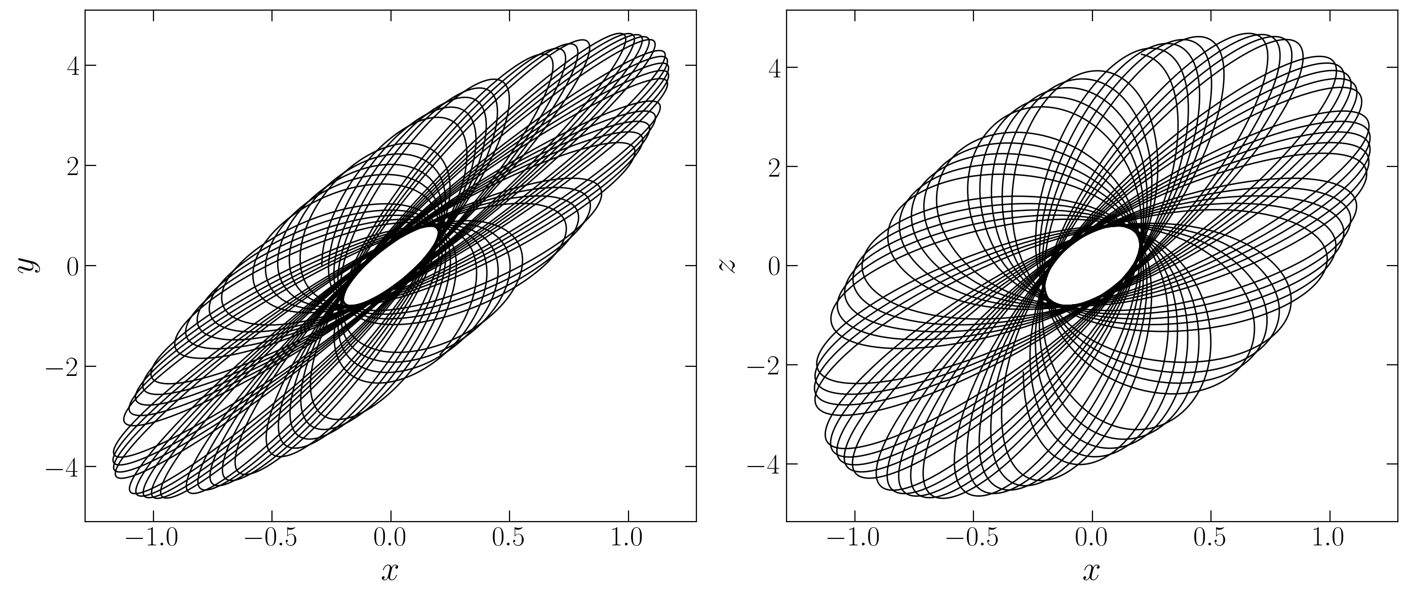
Plot orbit

orb = 1

# plot first 5_000 tsteps of the orbit
fig, axs = plt.subplots(1, 2, figsize=(14,6))

axs[0].plot(x[orb][:5_000], y[orb][:5_000], 'k-')
axs[0].set_xlabel(r'$x$')
axs[0].set_ylabel(r'$y$')
# axs[0].axis([-15, 15, -15, 15])

axs[1].plot(x[orb][:5_000], z[orb][:5_000], 'k-')
axs[1].set_xlabel(r'$x$')
axs[1].set_ylabel(r'$z$')
# axs[1].axis([-15, 15, -15, 15])

plt.tight_layout()

Spectrum

Total time and frequencies where spectrum is evaluated:

T = t[orb,-1] - t[orb,0]
omega = 2.*np.pi*np.fft.fftfreq(n_steps, T/n_steps)

# plot powew spectrum
# The limits can change for different orbits

fig, axs = plt.subplots(n_freqs, 2, figsize=(16,20))
fig.suptitle('Spectra before removal of kth freq.', fontsize=30)

axs[0,0].set_title(r'$r$', fontsize=36)
axs[0,1].set_title(r'$\varphi$', fontsize=36)
for i in range(n_freqs):
    axs[i,0].plot(np.fft.fftshift(omega), np.fft.fftshift(spec_r[orb,i]), '-', label=r'$k=%d$'%(i+1))
    axs[i,0].set_ylabel(r'$|a_r|$')
    axs[i,0].axis([-1, 1, -0.05, 1.])

    axs[i,1].plot(np.fft.fftshift(omega), np.fft.fftshift(spec_phi[orb,i]), '-', label=r'$k=%d$'%(i+1))
    axs[i,1].set_ylabel(r'$|a_\varphi|$')
    axs[i,1].axis([-1, 1, -0.05, 1.])

    for j in range(2):
        axs[i,j].set_xlabel(r'$\omega$')
        axs[i,j].legend(fontsize=24, loc=1)

plt.tight_layout()
fig.subplots_adjust(top=0.94, bottom=0.08, right=0.95, left=0.05, hspace=0.25, wspace=0.25)

Checking a specific peak

We now compare the first (raw) estimate of the peak frequency with the refined estimate obtained when we go to the continuum, i.e. by maximizing the function \(|\phi(\omega)| = \int_{-T/2}^{T/2} f(t)e^{-i\omega t}\chi_p(t)\, dt\), where \(f(t)\) is the time-series and \(\chi_p(t)\) is the window function:

k = 0 #kth frequency

# Calculate |phi(om)| at 1st raw maximum estimate om_max,
# at the edges of the interval om_inf, om_sup,
# and in intermediate points
tc = 0.5*(t[orb,0] + t[orb,-1])
# time symmetric around tc:
t_sym = t[orb] - tc
# window function:
chi = naif.chi_p(t_sym, p=1)
f_chi = fr[orb]*chi

# identify position of desired peak:
idx_max = np.argmax(spec_r[orb, k])
om_max = omega[idx_max]
# Define range around it, where to evaluate phi(omega):
om_inf = om_max - 4*np.pi/T
om_sup = om_max + 4*np.pi/T
# phi(om_max):
phi_om_max = -naif.mn_phi_om(om_max, f_chi, t_sym)

n_fine_om = 200
fine_om = np.linspace(om_inf, om_sup, n_fine_om)
# phi(omega):
fine_phi_om = np.zeros(n_fine_om)
for i in range(n_fine_om):
    fine_phi_om[i] = -naif.mn_phi_om(fine_om[i], f_chi, t_sym)

We now plot the function \(|\phi(\omega)|\) which is maximized to find the best estimate of the frequency at the peak. Vertical lines show the grid where the power spectrum is evaluated, used for the fist raw estimate. The peak of the black curve shows the improved (final) estimate. We do it for the radial component, for a certain orbit \(orb\) and around a certain peak \(k\):

# Plot
fig, axs = plt.subplots(1, figsize=(8,6))

axs.plot(fine_om, fine_phi_om, 'k-')
axs.plot(om_max, phi_om_max, 'r*', label='1st (raw) estimate')

best_omega, _ = naif.find_peak_freqs(fr[orb], t[orb])
axs.axvline(x=best_omega, c='k')
axs.plot(fine_om[np.argmax(fine_phi_om)], fine_phi_om[np.argmax(fine_phi_om)], 'k*', label='Final estimate')

axs.set_xlabel(r'$\omega$')
axs.set_ylabel(r'$|\phi(\omega)|$')
axs.legend(fontsize=20)

idx_max = np.argmax(np.fft.fftshift(spec_r[orb,k]))
omega_shift = np.fft.fftshift(omega)
for i in range(idx_max-2, idx_max+3):
    axs.axvline(x=omega_shift[i], c='r')

plt.tight_layout()